- How can I show & explain an application or service architecture?
- How can I draw “correct” (and what does that mean?) UML diagrams?
Let me show you how I document smallish software systems with, typically, no more than four UML diagrams. We'll cover the questions, what is worth diagramming? and what can I do with these diagrams anyway? and we'll cover enough UML to be useful.
I will use the example of developing a “lead generation” website, which should be simple enough to not get bogged down, but complex enough to answer some of the but how do I …? questions that more complex systems raise.
Why Diagrams?
Use diagrams as starting point to discuss, describe and explain your system. A diagram can give an instant overview of some aspect of the system. It can show important relationships on a single sheet of paper. It can raise important questions and show design decisions.
Why UML?
The UML is a visual modelling language. It has a vocabulary and grammar for diagramming software such that the diagram is a precise statement. So it can be used to show and explain software architecture.
The UML is the only diagramming standard left standing (with, perhaps, one exception that we'll see later). You may be tempted to compete in this uncrowded field of standards for software diagrams. I comment only that the UML contains several decades of work by several thoughtful people and if you can produce a usable standard that is simpler, quicker to learn, and not unhelpfully imprecise, then I shall be impressed.
You may also be tempted — as many, many of your colleagues have been — to just do without a standard. I hope these few examples will persuade you that learning a standard is less work than you fear and more useful than you expect.
Why 2+1 views?
The UML tells you how to diagram once you've decided what to diagram. “2+1” is a minimal decision about what to diagram. It suggests a couple of diagrams for the logical view of your software and one for the physical view (we'll explain what those words mean, too). That's the 2. But it starts with the 1, which is the context.
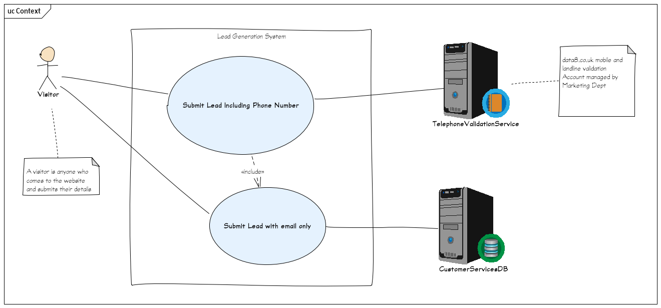
The System Context: Shown with a UML Use Case Diagram
Always start with context. Always start with simple.
The context diagram should make sense to your non-technical customer and can be so simple you wouldn't even give it a second glance. It shows:
- Who and what will use the system
- What the system will do
- Who and what the system will rely on
In the UML, anyone or anything who uses the system, or is relied on by the system to do its thing, is an Actor. What the system will do is a UseCase. A UseCase is a instance of the system being used to do something. It is shown on a diagram just by its name, which is a single descriptive phrase, in an ellipse.
- Anything inside the box is what the system does.
- Anything outside the box is the context of the system.
How to Use a Context / Use Case Diagram?
Use the diagram to discuss scope, expectations and dependencies with the system's customers and with the development team who will build it. Its simplicity and brevity should also clarify what is not (or not yet) expected of the system. Like user stories, the brevity calls for conversation to clarify. Complex Use Cases call for detailed careful business analysis too, but that is done with words, not pictures.
For your developers, this diagram is the high level overview of what they're delivering — everything inside the box — and what the system will need for it to work — everything outside the box.
I really like having a “hand drawn” look when first showing diagrams, because it says “work in progress” and invites participation. A precisely drawn diagram risks the impression of being a final decision.
I try to draw diagrams to be read from top left to bottom right. So I put “active” Actors—the users—on the left, and “dependency” actors on the right. That's not a part of UML, but it's part of how I will talk through the diagram.
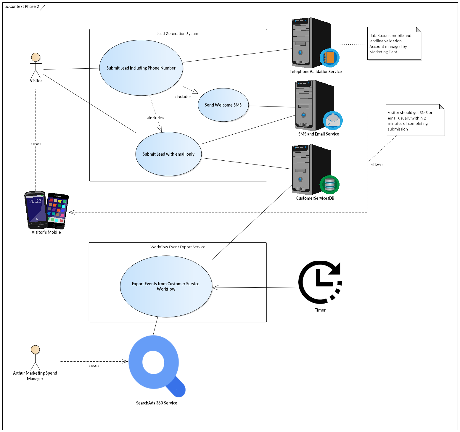
Here's the same diagram later on on the project. In phase two, we're giving visitors SMS feedback, and adding a whole new bit of functionality to read events from the customer service team and integrate then with web analytics.
What if you have lots of use cases? Don't put more on one diagram than you can usefully discuss in a single session. Pick out the main use cases & those that show the main external dependencies (which probably means, the ones that pose the highest risk to your project). Optionally, have a second diagram for all use cases, but only if you have an audience for it.
UML Definitions
There are 3 things you need to know for this diagram:
Actor, UseCase, and Subject aka System Boundary
Here are their definitions, which I've abbreviated from the UML 2.5 spec, section 18 Use Cases.
UseCases are a means to capture the requirements of systems, i.e., what systems are supposed to do. The key concepts specified in this clause are Actors, UseCases, and subjects. Each UseCase’s subject represents a system under consideration to which the UseCase applies. Users and any other systems that may interact with a subject are represented as Actors.
A UseCase is a specification of behavior. An instance of a UseCase refers to an occurrence of the emergent behavior that conforms to the corresponding UseCase. Such instances are often described by Interactions.
An Actor models a type of role played by an entity that interacts with the subjects of its associated UseCases (e.g., by exchanging signals and data). Actors may represent roles played by human users, external hardware, or other systems.
NOTE. An Actor does not necessarily represent a specific physical entity but instead a particular role of some entity that is relevant to the specification of its associated UseCases. Thus, a single physical instance may play the role of several different Actors and, conversely, a given Actor may be played by multiple different instances.
NOTE. The term “role” is used informally here and does not imply any technical definition of that term found elsewhere in this specification.
A UseCase is shown as an ellipse, either containing the name of the UseCase or with the name of the UseCase placed below the ellipse. An optional stereotype keyword may be placed above the name.
A subject for a set of UseCases (sometimes called a system boundary) may be shown as a rectangle with its name in the top-left corner, with the UseCase ellipses visually located inside this rectangle.
An Actor is represented by a “stick man” icon with the name of the Actor in the vicinity (usually above or below) the icon. An Actor may also be shown as a Classifier rectangle with the keyword «actor»
Other icons that convey the kind of Actor may also be used to denote an Actor, such as using a separate icon for non- human Actors.
The spec: https://www.omg.org/spec/UML
I have used 3 more UML features to add explanations:
- A Comment is “a textual annotation that can be attached to a set of Elements”. A Comment is shown as a rectangle with the upper right corner bent (this is also known as a “note symbol”). The rectangle contains the body of the Comment. The connection to each annotatedElement is shown by a separate dashed line. The dashed line connecting the note symbol to the annotatedElement(s) may be suppressed if it is clear from the context, or not important in this diagram.
- A Dependency “implies that the semantics of the clients are not complete without the suppliers”. A Dependency is shown as a dashed arrow between two model Elements. The model Element at the tail of the arrow (the client) depends on the model Element at the arrowhead (the supplier) .
- InformationFlows “describe circulation of information through a system in a general manner. They do not specify the nature of the information, mechanisms by which it is conveyed, sequences of exchange or any control conditions”. An InformationFlow is represented using the same notation as Dependency , with the keyword «flow» adorning its dashed line.