cafeenco – Chris F Carroll

Transcript of Prof. David Colquhoun, Oct 2020 talk at RIOT Science Club

https://www.youtube.com/watch?v=agC-SG5-Qyk

“Today I speak to you of war. A war that has pitted statistician against statistician for nearly 100 years. A mathematical conflict that has recently come to the attention of the normal people and these normal people look on in fear, in horror, but mostly in confusion because they have no idea why we're fighting.”
Kristin Lennox (Director of Statistical Consulting, Lawrence Livermore National Laboratory)

So that sums up a lot of what's been going on. The problem is that there is near unanimity among statisticians that p-values don't tell you what you need to know but statisticians themselves haven't been able to agree on a better way of doing things.

This talk is about the probability that if we claim to have made a discovery we'll be wrong. This is what people very frequently want to know. And that is not the p-value. You want to know the probability that you'll make a fool of yourself by claiming that an effect is real when in fact it's nothing but chance.

Just to be clear, what I'm talking about is how you interpret the results of a single unbiased experiment. Unbiased in the sense the experiment is randomized, and all the assumptions made in the analysis are exactly true. Of course in real life false positives can arise in any number of other ways: faults in the randomization and blinding, incorrect assumptions in the analysis, multiple comparisons, p-hacking and all of these things are going to make the risk of false positives even worse. So in a sense what I'm talking about is your minimum risk of making a false positive even if everything else were perfect.

The conclusion of this talk will be:

If you observe a p-value close to 0.05 and conclude that you've discovered something, then the chance that you'll be wrong is not 5%, but is somewhere between 20% and 30% depending on the exact assumptions you make. If the hypothesis was an implausible one to start with, the false positive risk will be much higher.

There's nothing new about this at all. This was written by a psychologist in 1966. The major point of this paper is that the test of significance does not provide the information concerning phenomena characteristically attributed to it, and that a great deal of mischief has been associated with its use. He goes on to say this is already well known, but if so it's not well known by many journal editors or indeed many users.

The p-value

Let's start by defining the p-value. An awful lot of people can't do this but even if you can do it it's surprisingly difficult to interpret it.

I consider it in the context of comparing two independent samples to make it a bit more concrete. So the p-value is defined thus:

If there were actually no effect—for example if the true means of the two samples were equal, so the difference was zero—then the probability of observing a value for the difference between means which is equal to or greater than that actually observed is called the p-value.

Now there's at least four things wrong with that when you think about it. It sounds very plausible but it's not.

“If there are actually no effect …”: first of all this implies that the denominator for the probability is the number of cases in which there is no effect and this is not known.
“… or greater than…” : why on earth should we be interested in values that haven't been observed? We know what the effect size that was observed was, so why should we be interested in values that are greater than that which haven't been observed?
It doesn't compare the hypothesis of no effect with anything else. This is put well by Sellke et al in 2001, “knowing that the data are rare when there is no true difference—that's what the p-value tells you—is of little use unless one determines whether or not they are also rare when there is a true difference”. In order to understand things properly, you've got to have, not only the null hypothesis but an alternative hypothesis.
The definition makes the error of the transposed conditional. That sounds a bit fancy but it's very easy to say what it is. The probability that you have four legs given that you're a cow is high but the probability that you're a cow given that you've got four legs is quite low many animals that have four legs that aren't cows. Take a legal example. The probability of getting the evidence given that you're guilty may be known. (It isn't of course — but that's the sort of thing you can hope to get). But it's not what you want. What you want is the probability that you're guilty given the evidence. The probability you're catholic given that you're the pope is probably very high, but the probability you're a pope given that you're a catholic is very low.

The nub of the matter

So now the nub of the matter: The probability of the observations given that the null-hypothesis is the p-value. But it's not what you want. What you want is the probability that the null-hypothesis is true given the observations.

https://www.youtube.com/watch?v=agC-SG5-Qyk#t=11m07

The first statement is a deductive process; the second process is inductive and that's where the problems lie. So these probabilities can be hugely different and transposing the conditional simply doesn't work.

The False Positive Risk

The false positive risk avoids these problems, if you define the false positive risk as follows:

If you declare a result to be “significant” based on a p-value after doing a single unbiased experiment, the False Positive Risk is the probability that your result is in fact a false positive.
time index 11m46

That, I maintain, is what you need to know. The problem is that in order to get it, you need Bayes theorem and as soon as that's mentioned, contention immediately follows.

The Likelihood Ratio

Suppose we call the null-hypothesis H₀, and the alternative hypothesis H₁. H₀ can be that the true effect size is zero and H₁ can be the hypothesis that there's a real effect, not just chance. So the odds on H₁ after you've done the experiment are equal to the likelihood ratio times the odds on there being a real effect before the experiment:

Odds on H₁ after experiment = Likelihood Ratio * Odds on H₁ before experiment

In general we would want a Bayes factor rather than the likelihood ratio, but that's the complication that my assumptions get round: we can use the likelihood ratio, which is a much simpler thing.

The likelihood ratio represents the evidence supplied by the experiment. It's what converts the prior odds to the posterior odds, in the language of Bayes' theorem. The likelihood ratio is a purely deductive quantity and therefore uncontentious. It's the probability of the observations if there's a real effect divided by the probability of the observations if there's no effect:

Likelihood Ratio= Pr[ observations | H₁ ] / Pr [ observations | H₀ ]

Notice a simplification you can make: if the prior odds equal 1, then the posterior odds are simply equal to the likelihood ratio. “Prior odds of 1” means that it's equally likely before the experiment that there was an effect or that there's no effect. That's probably the nearest you can get to declaring equipoise.

Comparison: Consider Screening Tests

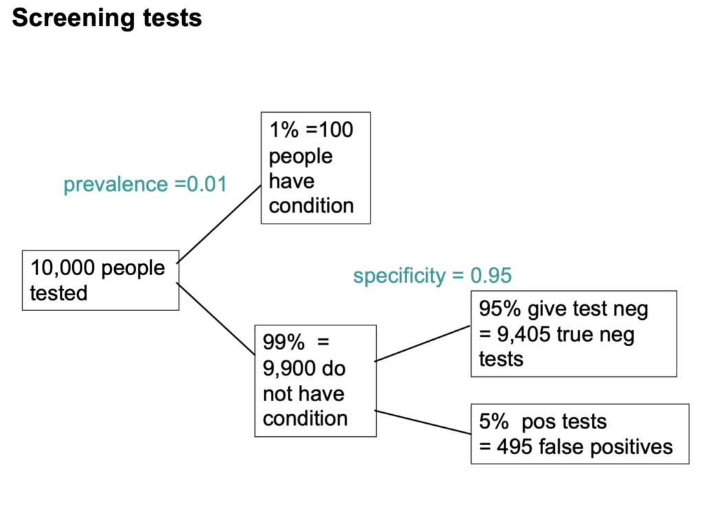
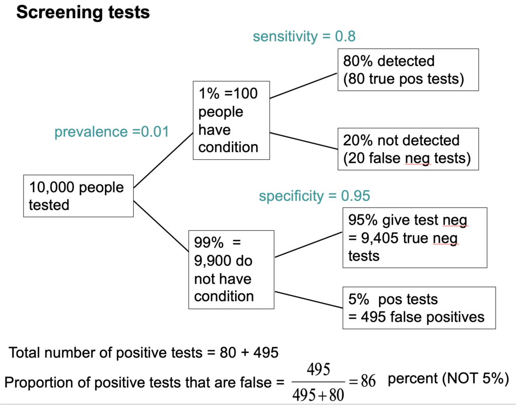
I wrote a statistics textbook in 1971 which by and large stood the test of time but the one thing I got completely wrong was the limitations of p-values. Like many other people I came to see these through thinking about screening tests. These are very much in the news at the moment and this is a an illustration of the problems they pose which is now quite commonplace.

Suppose you test 10,000 people and that 1 in a 100 of those people have the condition, say Covid, and 99 don't. So the prevalence in the population you're testing is 1 in a 100. So you have 100 people with the condition and 9,900 who don't. If the specificity of the test is 95%, you get 5% false positives. This is very much like a null-hypothesis test: it's a test of significance.

The Test of Significance: “there are only 5% false-positives”??

But you can't get the answer without considering the alternative hypothesis, which null-hypothesis significance tests don't do. You've got 1% (so that's 100 people) who have the condition, if the sensitivity of the test is 80%—that's like the power of a significance test—then you get to the total number of positive tests is 80 plus 495 and the proportion of tests that are false is 495 false positives on the total number of positives, which is 86%. 86% false positives is pretty disastrous. It's not 5%! Most people are quite surprised by that when they first come across it.

*But that* 5% means that 86% of all positives are false positives!

Now Look at Significance Tests In a Similar Way

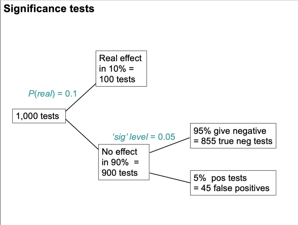
Now we can do something similar to significance tests though the parallel as I'll explain is not exact.

Suppose we do 1,000 tests and within 10% of them there's a real effect, and in 90% of them there is no effect. If the significance level, so-called, is 0.05 then we get 5% false positive tests, which is 45 false positives.

But that's as far as you can go with a null-hypothesis significance test. You can't tell what's going on unless you consider the other arm. If the power is 80% then we get 80 true positive tests and 20 false negative tests, so total number of positive tests is 80 plus 45 and the false discovery risk is the number of false positives divided by the total number of positives which is 36 percent.

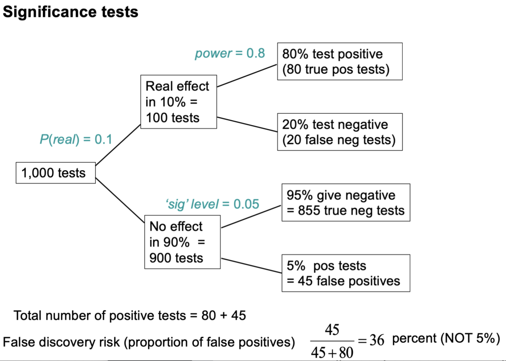
No. In the full picture, 36% of positives are false positives

So the p-value is not the false positive risk. The type-1 error rate is not the false positive risk.

The difference lies not in the numerator, it lies in the denominator. In that example of the 900 tests in which the null-hypothesis was true, there were 45 false positives. So looking at it from the classical point of view, the false positive risk would turn out to be 45 over 900 which is 0.05 but that's not what you want. What you want is the total number of false positives divided by the total number of positives which is 0.36.

The p-value is NOT the probability that your results occurred by chance. The false positive risk is.

As I said, the false positive risk in that case is 36%.

Complication: “p-equals” vs “p-less-than”

But now we have to come to a slightly subtle complication. It's been around since the 1930s and it was made very explicit by Dennis Lindley in the 1950s. It is unknown to most people which is very weird. The point is that there are two different ways in which we can calculate the likelihood ratio and therefore two different ways of getting the false positive risk.

A lot of writers including Ioannidis and Wacholder and many others use the “p less than” approach. That's what that tree diagram gives you. But it is not what is appropriate for interpretation of a single experiment. It underestimates the false positive risk.

What we need is the “p equals” approach, and I'll try and explain that now.

Suppose we do a test and we observe p=0.047 then all we are interested in is, how tests behave that come out with p=0.047. We aren't interested in any other different p-value. That p-value is now part of the data. The tree diagram approach we've just been through gave a false positive risk of only 6%, if you assume that the prevalence of true effects was 0.5 (prior odds of 1). 6% isn't much different from 5% so it might seem okay.

But the tree diagram approach, although it is very simple, still asks the wrong questions. It looks at all tests that gives p ≤ 0.05, the “p-less-than” case. If we observe p=0.047 then we should look only at tests that give p=0.047 rather than looking at all tests which could be equal to or less than 0.05. If you're doing it with simulations of course as in my 2014 paper then you can't expect any tests to give exactly 0.047; what you can do is look at all the tests that come out with p in a narrow band around there, say 0.045 ≤ p ≤ 0.05.

This approach gives a way of looking at the problem. It gives a different answer from the tree diagram approach. If you look at only tests that give p-values between 0.045 and 0.05, the false positive risk turns out to be not 6% but at least 26%. I say at least, because that assumes a prior probability of there being a real effect of 50:50.

If only 10% of the experiments had a real effect of (a prior of 0.1) in the tree diagram this rises to a disastrous 76% of false positives. That really is pretty disastrous. Now of course the problem is you don't know this prior probability.

The numbers that I got in the 2014 simulation paper, had a p-less-than approach claiming a false positive risk of about 6%, but a p-equals analysis tells us, under the null-hypothesis, the chance of getting a p-value between 0.045 and 0.05 is much smaller, and that the false positive risk is more like 26%.

The likelihood-ratio approach with two hypotheses

The problem with Bayes theorem is that there exists an infinite number of answers. Not everyone agrees with my approach, but it is one of the simplest.

I look at the likelihood ratio—that is to say, the relative probabilities of observing the data given two different hypotheses. One hypothesis is the zero effect (that's the null-hypothesis) and the other hypothesis is that there's a real effect of the observed size. That's the maximum likelihood estimate of the real effect size. Notice that we are not saying that the effect is exactly zero; but rather we are asking whether a zero effect explains the observations better than a real effect.

Now this amounts to putting a “lump” of probability on there being a zero effect. If you put a prior probability of 0.5 for there being a zero effect, you're saying the prior odds are 1. If you are willing to put a lump of probability on the null-hypothesis, then there are several methods of doing that. They all give similar results to mine within a factor of two or so.

EJ Wagenmakers sums it up in a tweet: “at least Bayesians attempt to find an approximate answer to the right question instead of struggling to interpret an exact answer to the wrong question” — that being the p-value.

Some actual results. First, the false positive risk as a function of the observed p-value.

The slide at time index 2 6 m05 is designed to show the difference between the “p-equals” and the “p-less than” cases:

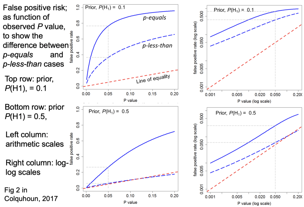
The top row shows what you get with a prior probability of 0.1.
The bottom row shows the prior probability of 0.5.
False positive risk is plotted against the p-value.

On each diagram the dashed red line is the “line of equality” that's where the points would lie if the p-value were the same as the false positive risk. Tou can see that in every case the blue lines—the false positive risk—is greater than the p value. For a prior probability of 0.5 then the false positive risk is about 26% when p=0.05.

So from now on I should use only the “p-equals” calculation which is clearly more relevant to a test of significance.

Now another set of graphs at time 27m46, for the false positive risk as a function of the observed p-value, but this time we'll vary the number in each sample. These are all for comparing two independent samples:

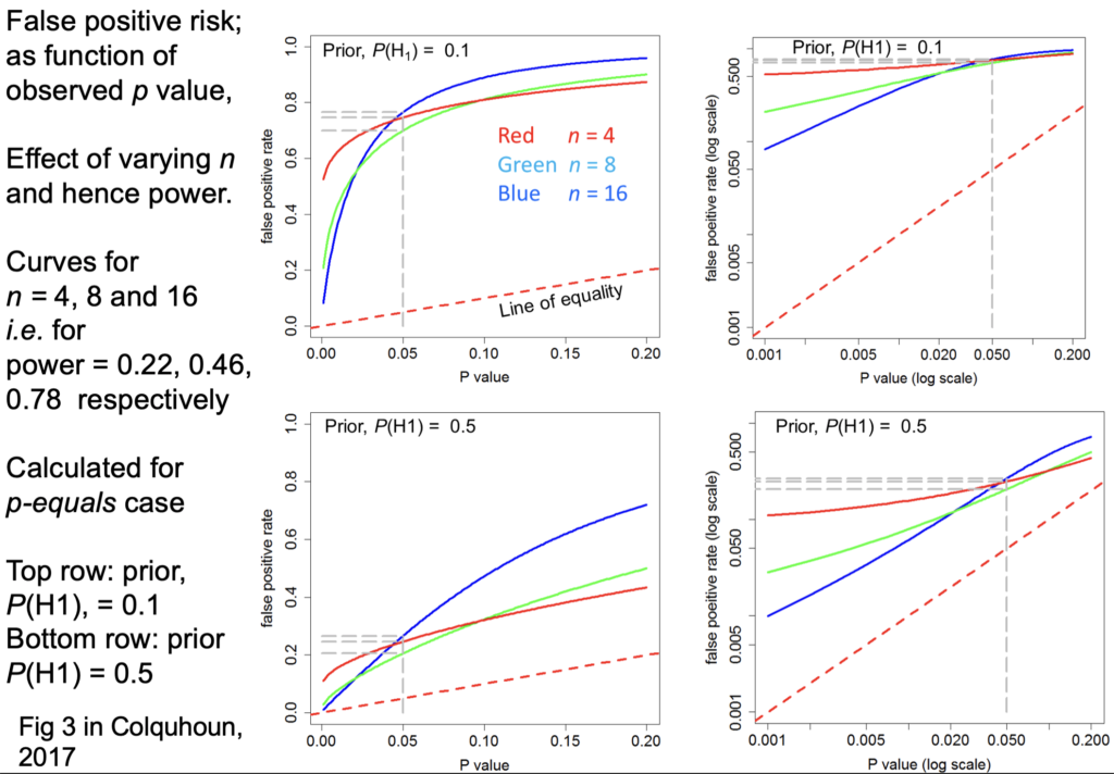
Focus on the log-log plot for prior of 0.5 in the bottom-right corner

Let's just concentrate on this log-log plot for a prior of 0.5. The curves are red for n=4 ; green for n=8 ; blue for n=16.

The top row is for an implausible hypothesis with a prior of 0.1, the bottom row for a plausible hypothesis with a prior of 0.5.

The power these lines correspond to is:
- n=4 has power 22%
- n=8 has power 46%
- n=16 that's the blue one has power 78%

Now you can see these behave in a slightly curious way. For most of the range it's what you'd expect: n=4 gives you a higher false positive risk than n=8 and that still higher than n=16 the blue line. It behaves in an odd way around 0.05;
they actually begin to cross. But the point is that in every case they're above the line of equality, so false positive risk is much bigger than the p-value in any circumstance.

Now the really interesting one: When I first did the simulation study I was challenged by the fact that the false positive risk actually becomes 1 if the experiment is a very powerful one. That seems a bit odd.

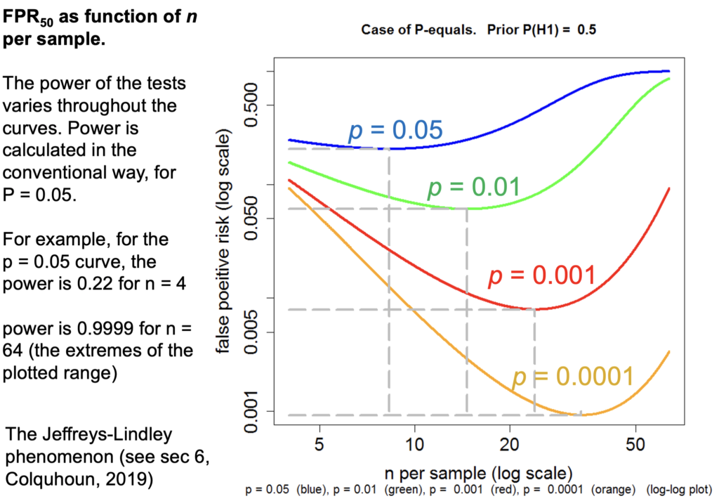
This is a false positive risk FPR₅₀ by which I mean “The False Positive Risk for prior odds of 1”, or a 50:50 chance of being a real effect or not a real effect.

Let's just concentrate on the p=0.05 curve and because the number per sample is changing, the power changes throughout the curve. For example on this p=0.05 curve for n=4 (that's the lowest one) r is 0.22 but if we go to the other end of the curve, n=64, The power is 99.99 something not achieved very often in practice.

But how is it p=0.05 can give you a false positive risk which approaches 100% even with p=0.01? It will eventually approach a false positive risk of 100% if p=0.01 and even if p=0.001 (and the same with other p-values) though it does so later and more slowly.
In fact this has been known for donkey's years. It's called the Jeffreys-Lindley paradox though there's nothing paradoxical about it: If the power is 99% then you expect almost every p-value to be very low. Everything is detected if we have a high power like that. In fact it would be very rare, with that very high power, to get a p-value as big as 0.05. Almost every p-value be much less than 0.05, and that's why p=0.05 would in that case provides strong evidence for the null-hypothesis. Even p=0.01 would provide strong evidence because almost every p-value with that would be much less than 0.01. This is a direct consequence of using the “p equals” definition which I think is what one ought to do. So the Jeffreys-Lindley phenomenon makes absolute sense.

Example

Now let's consider an actual practical example. This is a study of transcranial electromagnetic stimulation published in Science magazine (so a bit suspect to begin with), and it concludes that an improved associated memory performance was produced by transcranial electromagnetic stimulation, p=0.043. In order to find out how big the sample sizes were I had to dig right into the supplementary material. It was only 8. Nonetheless let's assume that they had an adequate power and see what we make of it:

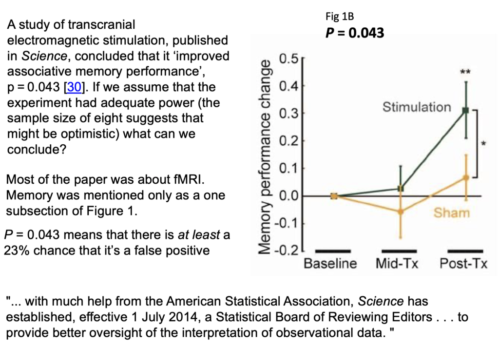
In fact it wasn't done in a proper parallel group way, it was done as before and after the stimulation and stab sham stimulation, and it produces one lousy asterisk. In fact most of the paper was about functional magnetic resonance imaging, this was only mentioned as a subsection of figure 1, but this is what was tweeted out because it sounds more dramatic than other things and it got a vast number of retweets. Now according to my calculations p=0.043 means there's at least a 23% chance that it's false positive.

How better might we express the result of this experiment?

We could say that the increase in memory performance was 1.88 ± 0.85 (SEM) with confidence interval 0.055 to 3.7 (extra words recalled on a baseline of about 10). Thus p = 0.043. This implies a false positive risk (i.e. the probability that the results occurred by chance only) of at least 18% so the result is no more than suggestive.

There are several other ways you can put the same idea. I don't like them as much but, you could say that the increase in performance gave p=0.043, and in order to reduce the false positive risk to 0.05 it would be necessary to assume that the prior probability of there being a real effect was 81%. You'd have to be almost certain that there was a real effect before you did the experiment before that result became convincing. Since there's no independent evidence that that's true, the result is no more than suggestive.

Or you could put it this way: the increase in performance gave p=0.043. In order to reduce the false positive risk to 0.05 it would have been necessary to observe p=0.0043, so the result is no more than suggestive.

The reason I now prefer the first of these possibilities is because the other two involve an implicit threshold of 0.05 for the false positive risk and that's just as daft as assuming a threshold of 0.05 for the for the p-value.

You can calculate these very easily with our web calculator [for latest links please go to http://www.onemol.org.uk/?page_id=456]. There are three options : if you want to calculate the false positive risk for a p-value and prior, we can put in the observed p-value 0.049, the prior probability, the real effect 0.5, the normalized effect size 1 standard deviation, number in each sample and the output panel updates itself automatically.

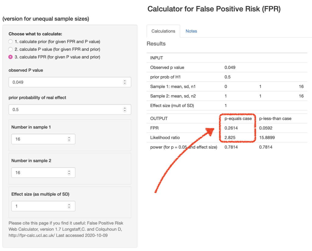
We see that the false positive risk for the “p-equals” case is 0.26 and the likelihood ratio is 2.8 (I'll come back to that in a minute). This sort of table can be very quickly calculated using the calculator or using the R programs which are provided with the papers:

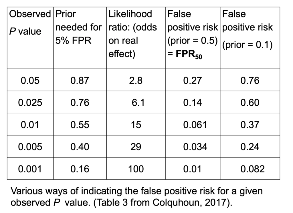
If we observe p=0.05, then it implies all the other things on this line: the prior probability that you need to postulate to get a 5% false positive risk would be 87%. You'd have to be almost ninety percent sure there was a real effect before the experiment, in order to to get a 5% false positive risk. The likelihood ratio comes out to be about 3; what that means is that your observations will be about 3 times more likely if there was a real effect than if there was no effect. 3:1 is very low odds compared with the 19:1 odds which you might incorrectly infer from p=0.05. The false positive risk for a prior of 0.5—the sort of default value which I call the FPR₅₀—would be 27% when you observe p=0.05.

In fact these are just directly related to each other. Since the likelihood ratio is a purely deductive quantity, we can regard FPR₅₀ as just being a transformation of the likelihood ratio and regard this as also a purely deductive quantity. For example, 1 - 2.8/(1+2.8) = 0.263, the FPR₅₀. Although in order to interpret it as a posterior probability then you do have to go into Bayes theorem. If the prior probability of a real effect was only 0.1 then that would correspond to a 76% false positive risk when you'd observed p=0.05. If we go to the other extreme, when we observe p=0.001 the likelihood ratio is 100 —notice not 1000, but 100— and the false positive risk would be 1%. That sounds okay but if it was an implausible hypothesis with only a 10% prior chance of being true, then the false positive risk would even then be above 5%, it would be 8% even when you observe p=0.001. In fact, to get this down to 0.05 you'd have to observe p=0.00043, and that's good food for thought.

So what do you do to prevent making a fool of yourself?

Never use the words significant or non-significant and then don't use those pesky asterisks please, it makes no sense to have a magic cut off. Just give a p-value.
Don't use bar graphs. Show the data as a series of dots.
Always remember, it's a fundamental assumption of all significance tests that the treatments are randomized. When this isn't the case, you can't expect an accurate result from a test.
So I think you should still state the p-value and an estimate of the effect size with confidence intervals but be aware that this tells you nothing very direct about the false positive risk. The p-value should be accompanied by an indication of the likely false positive risk. It won't be exact but it doesn't really need to be; it does answer the right question. You can for example specify the FPR₅₀, the false positive risk based on a prior probability of 0.5. That's really just a more comprehensible way of specifying the likelihood ratio. You can use other methods, but they all involve an implicit threshold of 0.05 for the false positive risk. That isn't desirable.

So p=0.04 doesn't mean you discovered something, it means it might be worth another look. In fact even p=0.005 can under some circumstances be more compatible with the null-hypothesis than with there being a real effect.

So this doesn't leave Fisher looking very good. Matthews (1988) said, “the plain fact is that 70 years ago Ronald Fisher gave scientists a mathematical machine for turning boloney into breakthroughs and flukes into funding”. Though it's not quite fair to blame R.A.Fisher because he himself described the 5% point as a quite a low standard of significance.

Q&A

Q: “There are lots of competing ideas about how best to deal with the issue of statistical testing. For the non-statistician it is very hard to evaluate them and decide on what is the best approach. Is there any empirical evidence about what works best in practice? For example, training people to do analysis in different ways, and then getting them to analyze data with known characteristics. If not why not? It feels like we wouldn't rely so heavily on theory in e.g. drug development, so why do we in stats?

A: The gist: why do we rely on theory and statistics? Well, we might as well say, why do we rely on theory in mathematics? That's what it is! You have concrete theories and concrete postulates. Which you don't have in drug testing, that's just empirical.

Q: Is there any empirical evidence about what works best in practice, so for example training people to do analysis in different ways? and then getting them to analyze data with known characteristics and if not why not?

A: Why not: because you never actually know unless you're doing simulations what the answer should be. So no, it's not known which works best in practice. I think you can rely on the fact that a lot of the alternative methods give similar answers. That's why I felt justified in using rather simple assumptions for mine, because they're easier to understand and the answers you get don't differ greatly from much more complicated methods.

In my 2019 or 2017 paper there's a comparison of three different methods, all of which assume that it's reasonable to test a point (or small interval) null-hypothesis (one that says that treatment effect is exactly zero), but given that assumption, all the alternative methods give similar answers within a factor of two or so. A factor of two is all you need: it doesn't matter if it's 26% or 52% or 13%, the conclusions in real life are much the same.

So I think you might as well use a simple method. There is an even simpler one than mine actually, proposed by Berger and Sellke that gives a very simple calculation from the p-value and that gives I think a false positive risk of 29 percent when you observe p=0.05. Mine method gives 26%, so there's no essential difference between them. It doesn't matter which you use really.

Q: The last question gave an example of training people so maybe he was touching on how do we teach people how to analyze their data and interpret it accurately. Reporting effect sizes and confidence intervals alongside p-values has been shown to improve interpretation in teaching contexts. I wonder whether in your own experience that you have found that this helps as well? Or can you suggest any ways to help educators, teachers, lecturers, to help the next generation of researchers properly?

A: Yes I think you should always report the observed effect size and confidence limits for it. But be aware that confidence intervals tell you exactly the same thing as p-values and therefore very suspect. There's a simple one-to-one correspondence between p-values and confidence limits. So if you use the criterion, “the confidence limits exclude zero difference” to judge whether there's a real effect you're making exactly the same mistake as if you use p≤0.05 to to make the judgment. So they they should be given for sure, because they're sort of familiar but you do need, separately, some sort of a rough estimate of the false positive risk too.

Q: I'm struggling a bit with the “p-equals” intuition. How do you decide the band around 0.047 to use for the simulations? Presumably the results are very sensitive to this band. If you are using an exact p-value in a calculation rather than a simulation, the probability of exactly that p-value to many decimal places will presumably become infinitely small. Any clarification would be appreciated.

A: Yes, that's not too difficult to deal with: you've got to use a band which is wide enough to get a decent number in. But the result is not at all sensitive to that: if you make it wider, you'll get larger numbers but the result will be much the same. In fact, that's only a problem if you do it by simulation. If you do it by exact calculation it's easier, (I have a spare slide I can show if you if you want to that illustrates that). To do a 100,000 or a million t-tests with my R script in simulation, doesn’t take long. But it doesn't depend at all critically on the width of the interval; and in any case it's not necessary to do simulations, you can do the exact calculation.

Q: Even if an exact calculation can't be done—it probably can—you can get a better and better approximation by doing more simulations and using narrower and narrower bands around 0.047?

A: Yes that’s absolutely true yes. Yes, I did check it with a million occasionally. The slide at time 53m17.5 shows how you do the exact calculation:

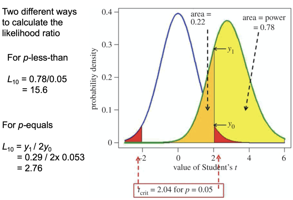
• The students t-value along the bottom
• Probability density at the side
• The blue line is the distribution you get under the null-hypothesis, with a mean of 0 and a standard deviation of 1 in this case.
• So the red areas are the rejection areas for a t-test.
• The green curve is the t-distribution (it’s a non-central t-distribution which is what you need in this case) for the alternative hypothesis. So it's centred round … (inaudible)
• The yellow area is the power, which here is 78%
• The orange area is (1-power) so 22%

Then they consider all values in the red area or in the yellow area as being positives. The p-equals hypothesis is, what you want is not the areas, but the ordinates here, the probability densities. The probability of getting a t-value of 0.04 under the null-hypothesis is that intercept and under (…inaudible…) so for the p-equals hypothesis, the likelihood ratio would be Y1/(2 * Y20) (2 because of the two red tails) and that gives you a likelihood ratio of 2.8. That corresponds to an FPR₅₀ of 26% as we explained. Now it's true that the probability of being in a narrow band around Y0 and Y1, would be zero, but the ratio of the two is perfectly well defined. It's not infinitesimal, in fact it's 2.8. So you can by calculation get the same result as you get from simulation. I hope that was reasonably clear. It may not have been if you aren't familiar with looking at those sorts of things.

Q: To calculate FPR₅₀—false positive risk for a 50:50 prior—I need to assume an effect size. Which one do you use in the calculator? Would it make sense to calculate FPR₅₀ for a range of effect sizes?

A: Yes if you use the web calculator or the R scripts then you want to specify what the normalized effect size is. You can use your observed one. If you're trying to interpret real data, you've got an estimated effect size. It's true (this was shown in the 2014 simulations of the 2017 exact calculations) that that likelihood ratio I gave of 2.8 when you observe p=0.05, that is done using the true effect size. All you've got is the observed effect size. So they're not the same of course. But you can easily show with simulations, that if you use the observed effect size in place of the the true effect size (which you don't generally know) then that likelihood ratio goes up from about 2.8 to 3.6 (from memory); it's around 3, either way. You can plug your observed normalised effect size into the calculator and you won't be led far astray.

Q: Consider hypothesis H₁ versus H₂ which is the interpretation to go with?

A: Well I'm not quite clear still what the two interpretations he's alluding to are but I shouldn't rely on the p-value interpretation. You can do a full Bayesian analysis. Some forms of Bayesian analysis can give results that are quite similar to the p-values. (That can't possibly be generally true because they make quite different assumptions). Stephen Senn produced an example where there was essentially no problem with p-value, but that was for a one-sided test with a fairly bizarre prior distribution.

In general in Bayes, you specify a prior distribution of effect sizes, what you believe before the experiment. Now, unless you have empirical data for what that distribution is, which is very rare, then I just can't see the justification for that. It's bad enough making up the probability that there's a real effect compared with there being no real effect. To make up a whole distribution just seems to be a bit like fantasy.

Mine is simpler because by considering a point null-hypothesis and a Point alternative hypothesis, what in general would be called Bayes factors become Likelihood Ratios. Likelihood ratios are much easier to understand than Bayes factors because they just give you the relative probability of observing your data under two different hypotheses. This is a special case of Bayes theorem. But as I mentioned, any approach to Bayes theorem which assumes a point null hypothesis gives pretty similar answers, so it doesn't really matter which you use.

There was edition of the American Statistician last year which had 44 different contributions about the world beyond p=0.05 and I find it a pretty disappointing edition because there was no agreement among people and a lot of people didn't get around to making any recommendation. They said what was wrong, but didn't say what you should do in response. The one paper that I did like was the one by James Berger and Sellke. They recommended their false positive risk estimate (as I would call it; they called it something different but that's what it amounts to) and that's even simpler to calculate than mine. It's a little more pessimistic, it can give a bigger false positive risk for a given p value, but apart from that detail, their recommendations are much the same as mine. It doesn't really matter which you choose.

Q: If people want a procedure that does not too often lead them to draw wrong conclusions, is it fine if they use a p-value?

A: No, that maximises your wrong conclusions, among the available methods! The whole point is, that the false positive risk is a lot bigger than the p-value under almost all circumstances. Some people refer to this as the p-value exaggerating the evidence; but it only does so if you incorrectly interpret the p value as being the probability that you're wrong. It certainly is not.

Q: Your thoughts on, there's lots of recommendations about practical alternatives to p-values. Most notably the Nature piece that was published last year—something like 400 signatories—that said that we should retire the p value. Their alternative was to just report effect sizes and confidence intervals. Now you've said you're not against anything that should be standard practice, but I wonder whether this alternative is actually useful, to retire the p-value?

A: I don't think the 400 author thing in nature recommended ditching p-values at all, it recommended ditching the 0.05 threshold, and just stating a p-value. That would mean abandoning the term “statistically significant” which is so shockingly misleading for the reasons I've been talking about. But it didn't say that you shouldn't give p-values, and I don't think it really recommended an alternative. I would be against not giving p-values because it's the p-value which enables you to calculate the equivalent false positive risk which would be much harder work if people didn't give the p-value.

If you use the false positive risk, you'll inevitably get a larger false negative rate. So, if you're using it to make a decision, other things come into it than the false positive risk and the p-value. Namely, the cost of missing an effect which is real, and the cost of getting a false positive. They both matter. If you can estimate the costs associated with either of them, then then you can draw some sort of optimal conclusion. But there aren't usually costs to getting a false positives. Certainly the costs of getting false positives or rather low for most people. In fact, there may be a great advantage to your career to publish a lot of false positives, unfortunately. This is the problem that the riot science club is dealing with I guess.

Q: What about changing the alpha level? To tinker with the alpha level has been popular in the light of the replication crisis, to make it even a more difficult test pass when testing your hypothesis. Some people have said that it should be 0.005 should be the threshold and

A: … Daniel Benjamin said that and a lot of other authors. I wrote to them about that and they said, they didn't really think it was very satisfactory but it would be better than the present practice. They regarded it as a sort of interim thing.

It's true that you would have fewer false positives if you did that, but it's a very crude way of treating the false positive risk problem. I would much prefer to make a direct estimate, even though it's rough, of the false positive risk rather than just crudely reducing to p=0.005. I do have a long paragraph in one of the papers discussing this particular thing. If for example you are testing a hypothesis about teleportation or mind-reading or homeopathy then you probably wouldn't be willing to give a prior of 50% to that being right before the experiment. In which case 0.005 would still be wrong, you would have to have a much lower p-value than that to get the false positive risk.

Author: cafeenco

Why p-values can’t tell you what you need to know and what to do about it